PID Drone Controller
A quadcopter flight controller simulated in CoppeliaSim and tuned in MATLAB — PID loops for position, velocity, and angular rate, with trajectory and step-response plots to check the gains.
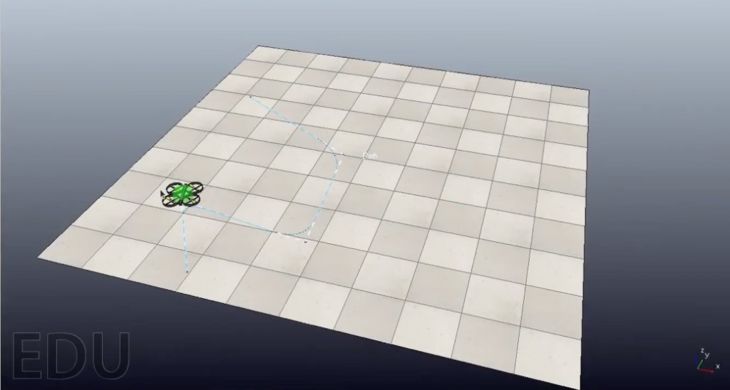
CoppeliaSim — quadcopter tracking a commanded path while the MATLAB PID loop runs
Role
Controls / simulation
Team
Individual
Status
Completed
Timeline
2025
- ▹CoppeliaSim plant + MATLAB control / analysis
- ▹PID on position, linear velocity, and angular velocity
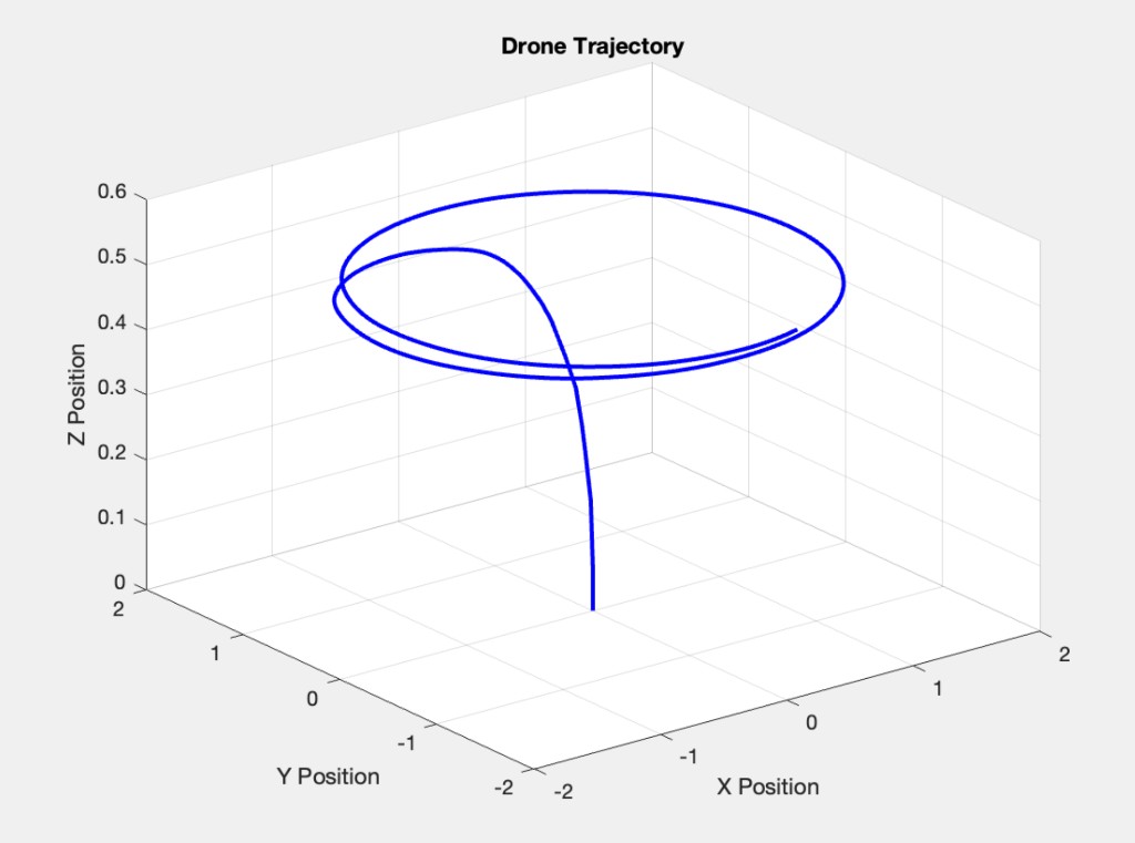
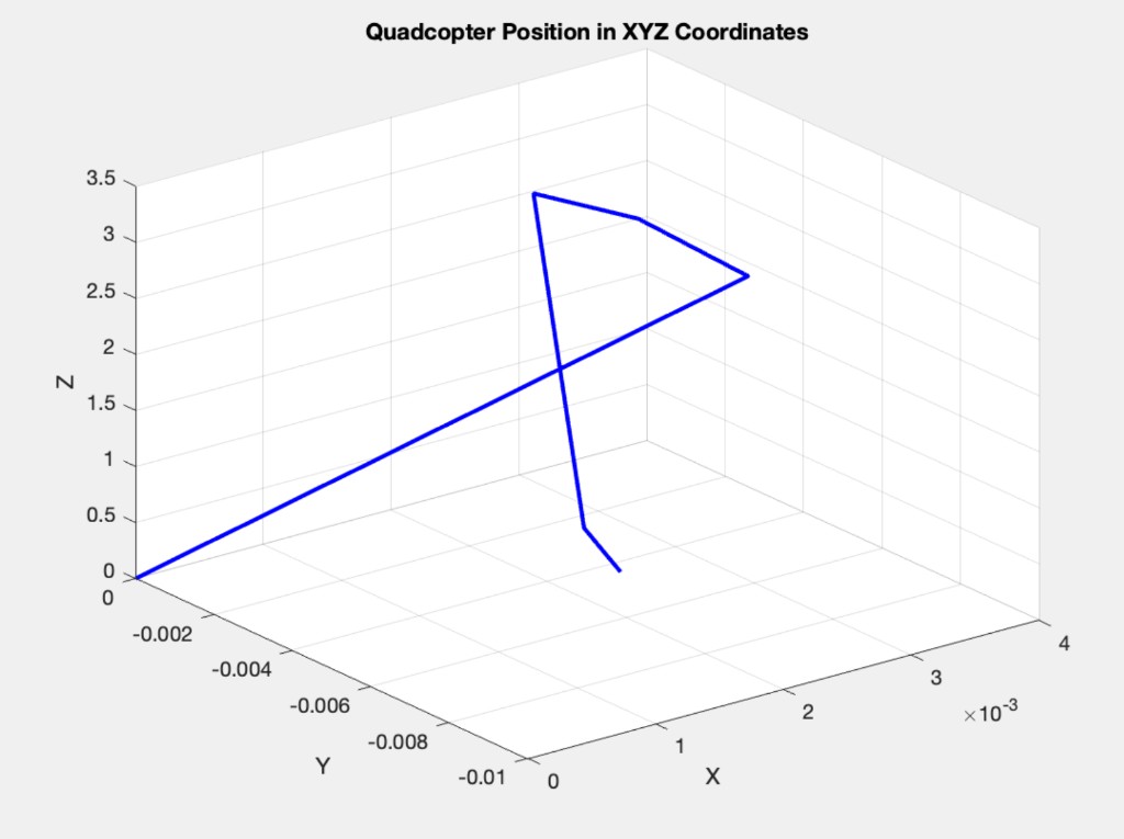
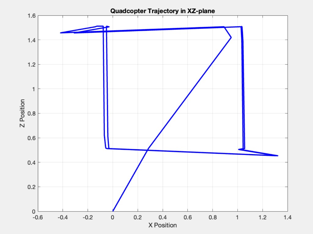
- ▹Simulated flight trajectories (orbit, XYZ, XZ plane)
- ▹Step-response plots to tune and verify gains
Overview
I built a PID flight controller for a simulated quadcopter using CoppeliaSim as the plant and MATLAB for control logic and analysis. The goal was to fly commanded paths and then use plots — trajectories plus step responses — to see how well the gains held position, velocity, and angular rate.
Simulation Setup
CoppeliaSim ran the drone model (motors, body dynamics, sensors). MATLAB closed the loop: read state, run PID, command motor speeds / setpoints, and log data for plotting.
Signals in the loop included: - Position (x, y, z) - Linear velocity - Angular velocity / yaw rate - Motor speed commands
I flew simple missions in sim — climb, hold altitude, orbit, and planar paths — then exported the logs into MATLAB figures.
PID Control
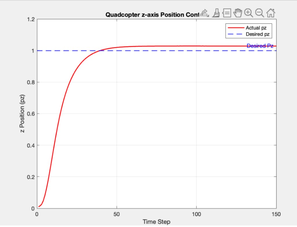
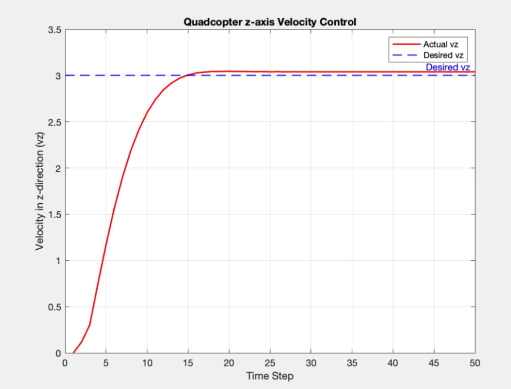
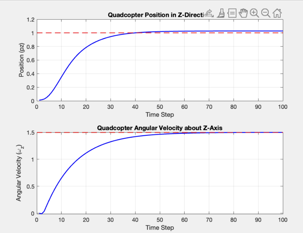
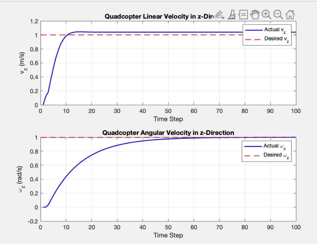
Separate (or cascaded) PID terms handled altitude, vertical velocity, and yaw rate, with gains tuned until the actual curves met the desired setpoints without wild overshoot.
The response plots compare actual vs desired for: - z position (pz) - z velocity (vz) - angular velocity about z (ωz)
Rise time, overshoot, and steady-state error were the usual checks while tweaking P, I, and D.
Trajectories
Three views of the flown path: - 3D orbit — takeoff, then a circular hold - XYZ path — full spatial maneuver - XZ plane — side view where corner overshoot shows the controller catching new setpoints
Results
The sim produced stable flights and clean tracking plots: altitude and velocity settled on the commanded lines, and the orbit / XZ paths matched the intended geometry closely enough to trust the gain set for classroom / lab use.
Lessons Learned
Simulation makes it safe to push gains hard, but you still need the plots — a path that “looks fine” in the 3D view can hide overshoot or slow settle that only shows up in the time-series.
Gallery
Questions about this project? Email Caleb.